http://www.rennes.archi.fr/grief.php
http://mpc-info-mpc.blogspot.com/
The so-called «Dragon» curve is a well known fractal curve, also known as the «Heighway» dragon, according to one of the NASA physicists (John Heighway, Bruce Banks, and William Harter) which are said to have first investigated it. It has been described By Martin Gardner in his Scientific American column «Mathematical Games» in 1967. It appears also on the section title pages of Jurassic Park by Michael Crichton, but moreover it plays a role in the plot, as one of the protagonists, mathematician and chaos theorist Ian Malcolm, creates dragon curves in order to simulate the actions that are to take place in the park, leading to its collapse (how exactly so, don’t ask me!).
I was reminded of this curve because this year (2012) is a Year of the Dragon in the 12-year cycle of the Chinese calendar. It is said to be the luckiest year in the Chinese Zodiac, so I hope it will contribute to an amelioration for a lot of people on earth that would need some...
In order to make my greeting card for this year, I combined the 2012 word with a dragon curve L-system. Instead of drawing a simple line, the R and L obtained by the rewriting system are interpreted as drawing the word 2012. As I went till the 12th step, there are 4096 «2012» in the last image. The previous step generates 2048 «2012»; too bad 2012 is not a power of 2; but remind me of doing a similar greeting card in 2048, more satisfyingly composed of 2048 «2048». I shall not be 100 years old yet, and the work is almost done, so I should be able to do it...
The Dragon Curve as L-system
The most common way to obtain a dragon curve is to use this L-system:
a=90°
axiom: L
L→L+R+
R→-L-R
It works, but you need to introduce some multiple of a 45° angle at the beginning of the drawing at each step, in order to obtain curves that match each other. If not, the successive curves turn around the starting point. So I prefer to use this L-system:
a=45°
axiom: L
L→-L++R-
R→+L—R+
You must also divide the length by √2 at each step in order to obtain the classical process. If you don’t divide the length, you obtain a growth process.
The dragon curve process is a folding process,which you can better demonstrate if you divide the length by 2 at each step, in order to maintain the whole length of the line. By the way, the dragon curve is easily done by hand by folding a long strip of paper in two, and by folding again the result (always in the same direction), and so on; and then by carefully partially unfolding this strip, all the angles having to be 90°.
The Dragon Curve and its variants as IFS
The dragon curve is also the attractor of this IFS:
| dragon curve | scaling | rotation | translation y | translation y |
| w1 | 1/√2 | 45° | 0 | 0 |
| w2 | 1/√2 | 135° | 1 | 0 |
The Dragon Curve and its variants as IFS
The dragon curve is also the attractor of this IFS:
| dragon curve | scaling | rotation | translation x | |
| translation y | ||||
| w1 | 1/√2 | 45° | 0 | 0 |
| w2 | 1/√2 | 135° | 1 | 0 |
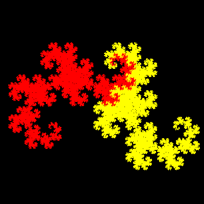
Fig. 1: the dragon as attractor of an IFS (chaotic algorithm)
The chaotic algorithm provides a thorough representation of the dragon curve, which actually covers a full portion of the plane, being of fractal dimension 2. We can also apply a deterministic algorithm to a starting set of points representing a line,which simulates the L-system. The description by the IFS leads to variants, considering that the dragon curve IFS consists of two transformations, each consisting of a scaling (ratio: 1/√2), composed with a rotation (angles 45° and 135° resp.) and a translation putting the two results side by side. Beyond the dragon curve itself, there are three possibilities, if we exclude those that are equivalent: the «crab» curve, the «triangle» curve, and the «twindragon» curve.
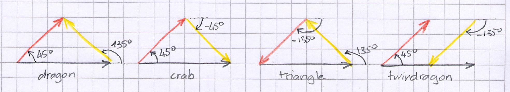
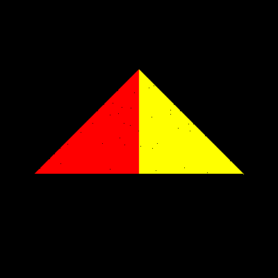
The 4 IFS may be described by the following schemes:
Fig. 2: schemes of the dragon IFS and its variants
The «crab» curve is obtained by this IFS:
| crab curve | scaling | rotation | translation x | translation y |
| w1 | 1/√2 | 45° | 0 | 0 |
| w2 | 1/√2 | -45° | .5 | .5 |
Fig. 3: the crab as attractor of an IFS (chaotic algorithm)
This curve is actually officially known as the Lévy C Curve, relating to French mathematician Pierre Paul Lévy. I choose to name it the crab curve here, because it looks like the eponymous zodiacal sign (also known as cancer, but it is not so joyful for obvious reasons) in western culture.
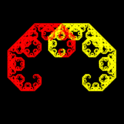
The «triangle» curve (its name is obvious) is obtained by this IFS:
| triangle curve | scaling | rotation | translation x | translation y |
| w1 | 1/√2 | -135° | .5 | .5 |
| w2 | 1/√2 | 135° | 1 | 0 |
Fig. 4: the triangle as attractor of an IFS (chaotic algorithm)
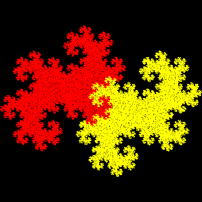
The «twindragon» curve is obtained by this IFS:
| twindragon curve | scaling | rotation | translation x | translation y |
| w1 | 1/√2 | 45° | 0 | 0w2 |
| w2 | 1/√2 | -135° | 1 | .5 |
Fig. 5: the twindragon as attractor of an IFS (chaotic algorithm)
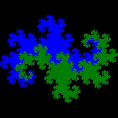
The «twindragon» curve is called this way, not because it would be a «twin» sister, a sibling, or even a «cousin» of the dragon curve, but because it is actually composed of two dragon curves, not as the red/yellow decomposition, but as this blue/green one:
Fig. 6: the twindragon as two dragons
Variants in L-system
The above schemes may also be interpreted in terms of L-systems. The angle is always 45°, the axiom always «L». When the arrow is in the right direction, it is interpreted as «L», when it is in the wrong direction, it is interpreted as «R».
Triangle curve:
L → -R++R-
R → +L--L+
Twindragon curve:
The scheme shows a difference: the two lines are not joined... One must introduce a new letter in the system, corresponding to a jump: J.
L→ -L+J+++L---J
J→ -J++J-
Varying the dimension
The dragon curve, as well as its variants, if of fractal dimension 2. It is easy to determine: each resulting figure is composed of 2 figures √2 smaller (and they have not got parts that are superposed, or not-contiguous, which is well shown in IFS chaotic results, where the two colours don’t mix, but touch somewhere). So its fractal dimension is equal to (log 2)/(log √2) = 2.
Varying the dimension consists in varying the angle a implied in the process. It is very straightforward in the L-systems, one has only to calculate the ratio of diminution of the length (2 cos a which, in the case of a=45°, is equal to √2). The respective fractal dimension of each curve is: (log 2)/(log (2cos a)), which varies from 1 (for a=0°) to 2 (for a=45°).
One notices that the triangle curve with a=30° is actually the well known Koch curve, though its construction is not the classical one, which skips every other step.
Hybridization
Hybridization consists in mixing two (or more) processes. This can be done in many ways. Here, I hybridize the dragon with the crab by using L-systems, with 14 steps. At each step, the algorithm chooses between the dragon rule (0) and the crab rule (1). There are 214 (= 16384) possible results. The animation shows this transition:
00000000000000
10000000000000
11000000000000
...
11111111111111
01111111111111
00111111111111
...
11111111111111
3D transposition
There are many ways in which we can think of a transposition of the dragon curve and its variants in 3D. The one I chose here considers the «skipped step» version suggested above, and is obtained by this L-system («&» and «^» stand for pitching up or down):
a=90°
axiom= A
A → -&A^AA+AA+AA^A&-
I call it the 3D crab, as it looks a lot like a crab!
;)